## Machine LearningThe goal of this part of the project is to improve the content relevance and user engagement with posts related to technical interviews on Reddit. By leveraging machine learning models such as Latent Dirichlet Allocation (LDA), which assigns a topic to each post, and K-Means clustering, showing us the different possible groupings based on a selected number of features chosen to group by, a clear analysis of the distribution of posts can be achieved. By utilizing the machine learning technical topics described on the home page, the topics associated with the different Reddit posts were found and able to be divided into 3 different categories, seemingly the most efficient number of categories given the data. A machine learning model was built to classify the usefulness of Reddit posts into groups of low, medium, or high usefulness based on upvote score, comment count, and text length. ### Topic 8: Text Classification*Goal:* Label posts as useful, semi-useful, or not useful through the use of text classification to provide job seekers guidance as to which characteristics contribute to a post’s engagement and, therefore, which discussions are most valuable for their study and preparation, allowing for focus on high-value content or shifting their focus elsewhere accordingly.##### 1) Determine Labels for Text ClassificationAs mentioned previously, the goal is to build a model that will identify novel Reddit posts and comments as useful, semi-useful, or not useful. In order to accomplish this, labels need to be assigned to the preexisting data. A usefulness label will be assigned to a comment or submission based on the following criteria:- Upvote/downvote score - This is possibly the best metric for measuring post usefulness. However, the meaning of an upvote on Reddit is oftentimes unclear. Upvotes are sometimes given to thank useful comments/submissions, but other times they're given as kudos to funny or clever comments/submissions. Therefore, by themselves they are not an ideal measure of usefulness.- Number of comments - In the case of submissions, this metric signifies the number of comments addressing the submission. For for comments themselves, this metric signifies the number of other comments addressing the same submission. This serves as a proxy for the importance of the overall discussion.- Length of text - As mentioned previously, upvotes are sometimes given as appreciation for witty or ironic comments that are not useful by the team's standards. These types of comments are often very short, so incorporating the length of the text into the label assignments will sift out comments that aren't useful and help ameliorate that problem.The first part in assigning the labels is to rescale each of these three variables from 0 to 1 using the following code:```{python}#| eval: False# Scale score, comment_count, and text_length to 0 to 1# Code referenced from https://stackoverflow.com/a/56953290/17331025from pyspark.ml.feature import MinMaxScalerfrom pyspark.ml.feature import VectorAssemblerfrom pyspark.ml import Pipelinefrom pyspark.sql.types import DoubleTypedf_scaled = df.alias('df_scaled')# UDF for converting column type from vector to double typeunlist = f.udf(lambda x: round(float(list(x)[0]),3), DoubleType())# Iterating over columns to be scaledfor i in ["score","comment_count", "text_length"]:# VectorAssembler Transformation - Converting column to vector type assembler = VectorAssembler(inputCols=[i],outputCol=i+"_vect")# MinMaxScaler Transformation scaler = MinMaxScaler(inputCol=i+"_vect", outputCol=i+"_scaled")# Pipeline of VectorAssembler and MinMaxScaler pipeline = Pipeline(stages=[assembler, scaler])# Fitting pipeline on dataframe df_scaled = pipeline.fit(df_scaled).transform(df_scaled).withColumn(i+"_scaled", unlist(i+"_scaled")).drop(i+"_vect")```Now, arbitrary weights are defined to assign to each of the three rescaled variables based on the subjective perception of the extent to which each one contributes to the overall usefulness of a submission or comment. The weights are designed as follows:- 1.0 for score since it is considered to be the most important- 0.8 for comment count it is considered to be somewhat important- 0.5 for text length since is it considered to be the least importantThus, a "label metric" is defined with the following formula:$LabelMetric = 1.0(Score) + 0.8(CommentCount) + 0.5(TextLength)$which yields the following distribution:```{python}#| eval: False# Define arbitrary weights for each of the three variables:lab_weights = [1, .8, .5] df_lab = df_scaled.withColumn('lab_metric', f.lit(lab_weights[0]) * f.col('score_scaled') + f.lit(lab_weights[1]) * f.col('comment_count_scaled') + f.lit(lab_weights[2]) * f.col('text_length_scaled'),)df_lab.select('lab_metric').summary().show()```| summary | lab_metric ||---------|------------|| count | 128345 || mean | 0.3089 || stddev | 0.1178 || min | 0.2092 || 25% | 0.2376 || 50% | 0.2662 || 75% | 0.3324 || max | 1.7658 |Based on the summary statistics of this label metric, the labels will be assigned according to these thresholds:| Label | Metric ||----------------------------------|---------------------------|| 2 - High usefulness/popularity | Greater than 0.3324 || 1 - Medium usefulness/popularity | Between 0.2662 and 0.3324 || 0 - Low usefulness/popularity | Less than 0.2662 |These thresholds roughly correspond to the 50th and 75th percentiles of the label metric. The rationale behind this decision is that Reddit is generally filled with many low-effort submissions and comments. The conservative assumptions are that about 50% of all submissions and comments will have low usefulness, 25% will have high usefulness, and the other 25% percent will be somewhere in the middle. The label metric calculated above is being used to assign these labels accordingly.The balance of labels can be seen below:```{python}#| eval: Falsedf_lab = df_lab.withColumn('label', f.when( f.col('lab_metric') >0.3324,2 )\ .when( f.col('lab_metric') <0.2662,0 )\ .otherwise(1))df_lab.groupBy('label').count().orderBy('label').show()```| label | count ||-------|-------|| 0 | 64133 || 1 | 32119 || 2 | 32093 |##### 2) Additional Data PreparationThe majority of the text cleaning was performed during the NLP phase, so at this point the only cleaning needed is to separate the text by whitespace and remove stopwords. In the code below, the pipeline is defined, a train-test split is performed, the model is trained, and six different values (0.0, 0.2, 0.4, 0.6, 0.8, 1.0) for the Naive Bayes smoothing hyperparameter $\alpha$ are tested.```{python}#| eval: False# This code was composed with the help of ChatGPT (primarily for identifying proper syntax)# Import librariesfrom pyspark.ml import Pipelinefrom pyspark.ml.feature import RegexTokenizer, StopWordsRemover, CountVectorizer, IDFfrom pyspark.ml.classification import NaiveBayesfrom pyspark.ml.evaluation import MulticlassClassificationEvaluatorfrom pyspark.ml.tuning import ParamGridBuilder, CrossValidator# Tokenizetokenizer = RegexTokenizer(inputCol="clean_body", outputCol="words", pattern="\\W")# Remove stopwordsstop_words_remover = StopWordsRemover(inputCol="words", outputCol="filtered_words")# TF-IDF vectorizationcv = CountVectorizer(inputCol="filtered_words", outputCol="raw_features")idf = IDF(inputCol="raw_features", outputCol="features")# Naive Bayes modelnb = NaiveBayes()# Pipelinepipeline = Pipeline(stages=[tokenizer, stop_words_remover, cv, idf, nb])# Train-test splittrain_data, test_data = df_model.randomSplit([0.8, 0.2], seed=123)# Hyperparameter tuning - test different alphas (smoothing parameter)paramGrid = (ParamGridBuilder() .addGrid(nb.smoothing, [0.0, 0.2, 0.4, 0.6, 0.8, 1.0]) .build())evaluator = MulticlassClassificationEvaluator(labelCol="label", predictionCol="prediction", metricName="accuracy")crossval = CrossValidator(estimator=pipeline, estimatorParamMaps=paramGrid, evaluator=evaluator, numFolds=5)# Fit modelcv_model = crossval.fit(train_data)# Make predictionspredictions = cv_model.transform(test_data)# Get accuracy and f1 scoreaccuracy = evaluator.evaluate(predictions)f1_score = MulticlassClassificationEvaluator(labelCol="label", predictionCol="prediction", metricName="f1").evaluate(predictions)print(f"Accuracy: {accuracy}")print(f"F1 Score: {f1_score}")```##### 3) Evaluate modelThe final performance of the model yields a validation accuracy of 0.5011 and F1 score of 0.4948. While these metrics indicate better performance than random guessing (which would, for example, theoretically produce an accuracy of 0.33), it is important to bear in mind that the system used for assigning labels is not perfect. The importance labels to the comments and submissions were assigned based on the team's own understanding of how Reddit works and what useful posts typically look like. This was a necessary approach given the scale of data, but if there was more time and resources, labels would most likely be manually assigned in order to ensure optimal performance in identifying useful posts. If this model were to be used in a practical application (for instance, to search Reddit for new posts that may be useful to job candidates), then the alternative approach of manually labeling each post in the training set would be preferred.<!-- 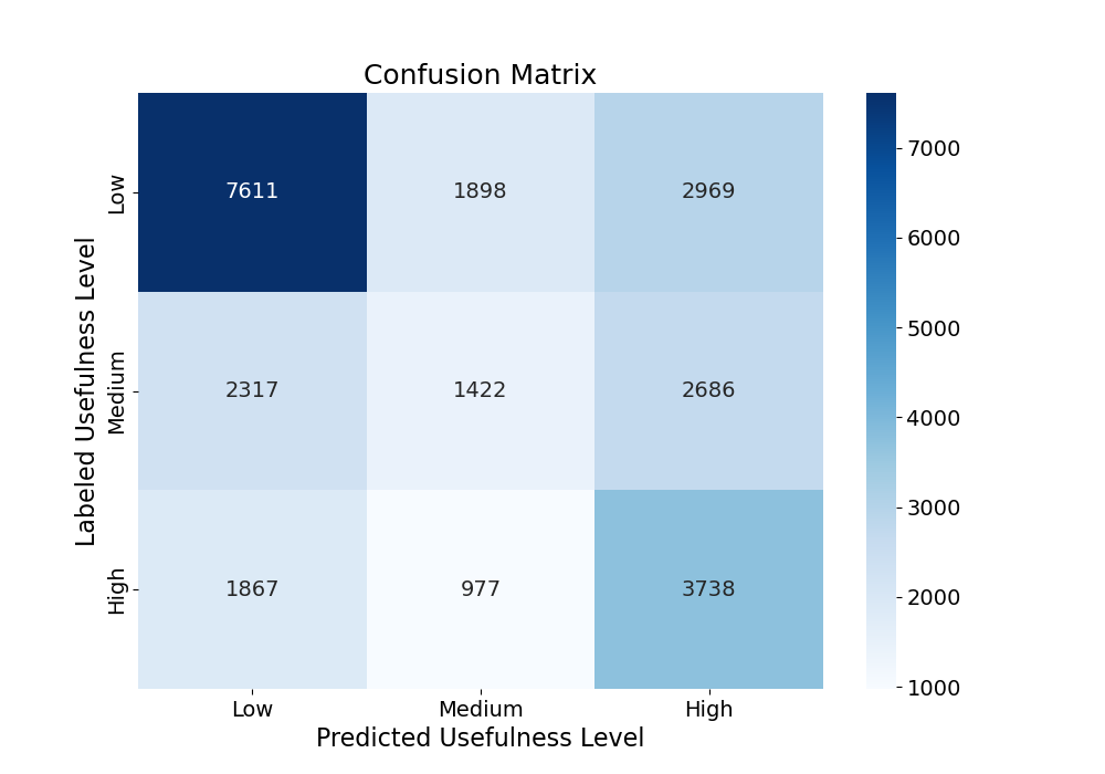 --><imgsrc="images/nb_confusion.png"style="width: 70%; height: auto;"/>The confusion matrix above further supports the need for a more robust system of labeling comments and submissions. The model predicts low-importance posts and high-importance posts relatively well, but clearly struggles at predicting semi-important posts. This is likely because the labeling system used left the semi-important label somewhat ambiguous. Where the low-importance and high-importance labels likely had their own distinct tokens to distinguish those labels, the posts labeled as semi-important likely had a mix of the two.### Topic 9: Topic Modeling*Goal:* Enhance the understanding of content themes in technical interview subreddits by applying Latent Dirichlet Allocation (LDA). This goal focuses on extracting concise and meaningful topics from the large amounts of text data from reddit, revealing trends in online discussions surrounding technical interviews.To find the clusters of the reddit post text data, an unsupervised learning technique may be used. LDA (Latent Dirichlet Allocation) is a popular unsupervised topic modeling method. With LDA, each "document", a post in this case, is assigned a "topic". Topics are comprised of several words that have associated weights. The weights are how likely the words belong to the gieven topic. Words with higher weights are the more "dominant" keywords for the given topic.As seen in the EDA section of this website, the reddit data was filtered on **7** "subreddits", essentially topics themselves. Can unsupervised machine learning produce similar topics, or do new topics arise? First, an LDA model with **7** topics will be trained to see how the topics compare to the subreddit topics and if any other noteable relationships arise. After this, LDA models with different amounts of topics will be trained to see if better results could be obtained.As a reminder, the **7** subreddits were:1. leetcode2. interviewpreparations3. codinginterview4. InterviewTips5. csinterviewproblems6. interviews7. big_tech_interviews#### LDA with 7 Topics**Terms by Topic:****Topic 1:** job, offer, company, interview, email, get, week, position, salary, time**Topic 2:** return, gt, int, array, node, lt, number, function, list, value**Topic 3:** problems, solve, leetcode, problem, lc, hard, solution, easy, solved, time**Topic 4:** deleted, interview, work, job, interviews, questions, people, youre, like, ask**Topic 5:** data, algorithms, coding, python, questions, structures, programming, learn, please, leetcode**Topic 6:** interview, good, job, got, said, like, know, thanks, really, asked**Topic 7:** solution, removed, question, problem, time, test, design, cases, dp, systemIt is clearly difficult to distinguish the topics as many contain the same and/or similar topic terms. The LDA was able to group the text into more general interview topics and more technical topics. For example, topics 2, 3 and 5 are the most technical topics out of the 7 with keywords like "leetcode" (one of the subreddits), "solution", "problem", "array", "function", etc. Topic 3 appears more general than topics 2 and 5. Topic 5 has a higher chance of having more detailed key words such as "algorithms" and "programming" while topic 2 contains keywords like "int", "array", "function", "list", "node", etc. Clearly, topic 2 would contain posts that are about specific coding problems that work with these data structures. Topic 1 contains the keywords "job", "offer", "company", "position", and "salary". Posts in this topic appear to be more about the logistics of interviewing - possibly questions about companies and the salaries of various positions, navigating accepting/declining a job offer, etc. Topics 4 and 6 appear to contain posts that are more about general interviewing, which is not surprising as a general "interviews" subreddit was used to filter the raw dataset. It is more difficult to differentiate between these two topics however. Topic 7 is similar to topics 4 and 6 but contains keywords "test", "design", and "cases", so this topic may contain posts that are more related to case interviews, test questions for interviews, etc. The plot below shows the top 10 keywords in each of the 7 topics. The bars represent each term's weight and are sorted from greatest to least.From the discussion above, it is clear that topic modelling with LDA can be challenging, especially with multiple topics that appear very similar. This unsupervised learning is an effective way to get more insight into the dataset, however, especially a dataset that may not be labelled in any way beforehand.```{python}#| eval: False# Import packagesimport timeimport sagemakerimport numpy as npimport pandas as pdimport pyarrow as paimport pyarrow.dataset as dsimport matplotlib.pyplot as pltimport pyLDAvis.gensim_models as gensimvisfrom gensim import corpora, modelsfrom s3fs import S3FileSystemfrom pyspark.sql import SparkSessionfrom pyspark.sql.functions import udffrom pyspark.sql.types import ArrayType, StringType, IntegerTypefrom sagemaker.spark.processing import PySparkProcessorfrom pyspark.ml.feature import Tokenizer, CountVectorizer, IDF, PCA, StopWordsRemoverfrom pyspark.ml.clustering import KMeans, LDAfrom pyspark.ml import Pipeline# Build Spark sessionspark = ( SparkSession.builder.appName("PySparkApp") .config("spark.jars.packages", "org.apache.hadoop:hadoop-aws:3.2.2") .config("fs.s3a.aws.credentials.provider","com.amazonaws.auth.ContainerCredentialsProvider", ) .getOrCreate())%%timesession = sagemaker.Session()#s3://sagemaker-us-east-1-131536150362/project/data_reformat_clean_nlp.parquet/bucket ="tm1450-project"output_prefix_data_submissions ="data_reformat_clean.parquet/"s3_path =f"s3a://{bucket}/{output_prefix_data_submissions}"print(f"reading data from {s3_path}")df = spark.read.parquet(s3_path, header=True)print(f"shape of the dataframe is {df.count():,}x{len(df.columns)}")## PREPARE THE DATA# Tokenize the texttokenizer = Tokenizer(inputCol ="clean_body", outputCol ="clean_body_tokenized")tokenized_df = tokenizer.transform(df)# Load english stopwordsstop_words = StopWordsRemover.loadDefaultStopWords("english")extra_stopwords = ["dont", "im", "a", "b", "c", "d", "e", "f", "g", "h", "i", "j", "k", "l", "m", "n", "o", "q", "r", "s", "t", "u", "v", "w", "x", "y", "z", "0", "1", "2", "3", "4", "5", "6", "7", "8", "9"]# Remove stop words from tokenized columnstop_remover = StopWordsRemover(inputCol ="clean_body_tokenized", outputCol ="clean_body_no_stop", stopWords = stop_words+extra_stopwords)tokenized_df_no_stop = stop_remover.transform(tokenized_df)# Vectorize the columncount_vectorizer = CountVectorizer(inputCol ="clean_body_no_stop", outputCol ="cv_features", vocabSize =5000, minDF =10.0)cv_model = count_vectorizer.fit(tokenized_df_no_stop)vocabulary = cv_model.vocabulary # Store the vocabularycv_df = cv_model.transform(tokenized_df_no_stop)# TF-IDFidf = IDF(inputCol ="cv_features", outputCol ="features")idf_model = idf.fit(cv_df)final_df = idf_model.transform(cv_df) ## FIT LDA MODEL AND GET THE TOPICSnum_topics =7# Define model with num_topics and fitlda = LDA(k = num_topics, maxIter =100)lda_model7 = lda.fit(final_df.select("features"))lda_df7 = lda_model7.transform(final_df)# View resultstopics7 = lda_model7.describeTopics(maxTermsPerTopic =10)topics7.show(truncate =True)# Get the keywords for each of the topicskeywords_by_topic7 = topics7.rdd.map(lambda row: row["termIndices"]).map(lambda indices: [vocabulary[idx] for idx in indices]).collect()# Get the term weights for each topicterm_weights_by_topic7 = topics7.select("termWeights").rdd.flatMap(lambda x: x).collect()# Print out the keywords by topicfor i, words inenumerate(keywords_by_topic7):print(f"Topic {i+1}: {', '.join(words)}") # Plotting keywords for each topicplt.figure()for i inrange(num_topics): plt.subplot(((num_topics +4-1)//4), 4, i +1) plt.barh(range(len(keywords_by_topic7[i])), term_weights_by_topic7[i], color ="#251279", alpha =1) plt.yticks(range(len(keywords_by_topic7[i])), keywords_by_topic7[i]) plt.title(f"Topic {i+1}") plt.xlabel("Keyword") plt.gca().invert_yaxis()plt.tight_layout()# Save figureplt.savefig('../../website-source/images/lda_plot_7_topics.png', dpi =300)plt.show()```<!--  --><imgsrc="images/lda_plot_7_topics.png"style="width: 70%; height: auto;"/>#### LDA with 3 TopicsNow, the LDA will be trained with fewer topics to see if it becomes easier to differentiate between the topics.**Terms by Topic:****Topic 1:** interview, job, company, get, like, interviews, work, deleted, know, ask**Topic 2:** solution, return, array, gt, code, int, problem, number, removed, use**Topic 3:** problems, leetcode, questions, solve, problem, data, coding, lc, algorithms, learnWith only 3 topics, it is clearly easier to distinguish between topics. The set of likely keywords in topic 1 show that posts classified into this topic are most likely about general interview questions, interview advice, discussion about companies in the industry, and more. Topic 2 on the other hand contains more technical keywords such as "int", "array", "solution", and "code." This topic probably contains posts about specific coding interview/assessment questions. Topic 3 is also technical, but more general than topic 2, containing likely keywords such as "leetcode" (one of the subreddits), "questions", "solve", "algorithms", "learn." Posts under this topic are probably also asking about coding interviews, what questions may come up, the best ways to prepare and "learn", etc. Leetcode is a popular website to practice for coding interviews, so this makes sense.```{python}#| eval: Falsenum_topics =3# Define model with num_topics and fitlda = LDA(k = num_topics, maxIter =100)lda_model3 = lda.fit(final_df.select("features"))lda_df3 = lda_model3.transform(final_df)# View resultstopics3 = lda_model3.describeTopics(maxTermsPerTopic =10)topics3.show(truncate =True)# Get the keywords for each of the topicskeywords_by_topic3 = topics3.rdd.map(lambda row: row["termIndices"]).map(lambda indices: [vocabulary[idx] for idx in indices]).collect()# Get the term weights for each topicterm_weights_by_topic3 = topics3.select("termWeights").rdd.flatMap(lambda x: x).collect()# Print out the keywords by topicfor i, words inenumerate(keywords_by_topic3):print(f"Topic {i+1}: {', '.join(words)}") # Plotting keywords for each topicplt.figure()for i inrange(num_topics): plt.subplot(((num_topics +4-1)//4), 4, i +1) plt.barh(range(len(keywords_by_topic3[i])), term_weights_by_topic3[i], color ="#251279", alpha =1) plt.yticks(range(len(keywords_by_topic3[i])), keywords_by_topic3[i]) plt.title(f"Topic {i+1}") plt.xlabel("Keyword") plt.gca().invert_yaxis()plt.tight_layout()# Save figureplt.savefig('../../website-source/images/lda_plot_3_topics.png', dpi =300)plt.show()```<!-- 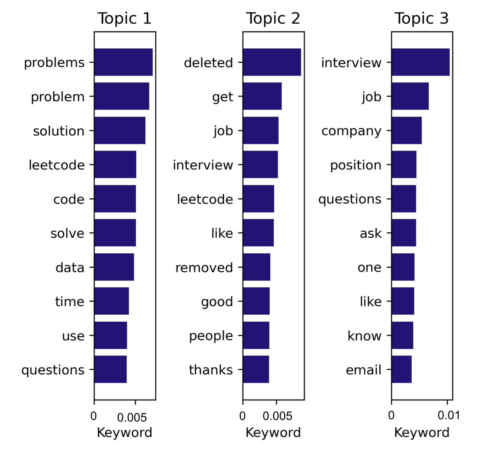 --><imgsrc="images/lda_plot_3_topics.png"style="width: 60%; height: auto;"/>Ultimately, LDA is a fantastic way to initially organize a dataset into different topics. In this case, LDA was performed to see if the learned topics were similar to the subreddits used to initially filter the dataset. Additionally, there was a desire to test if any new topics arise.The topics do seem to align with the subreddits: more general subreddits such as "interview" and "InterviewTips" and more technical/specific subreddits such as "leetcode" and "codinginterview." Similar categorizations were seen in the learned topics from LDA. As the subreddits used to filter the data were already very specific to interviews, in particular technical and coding interviews, no new topics appeared to arise through LDA.### Topic 10: Post Clustering*Goal:* Discover underlying themes in subreddit discussions by applying K-means clustering. This method aims to segment posts and comments into distinct clusters based on the content of the text. This presents an opportunity to offer a new perspective on strong topics and conversation patterns within the technical interview reddit community.The code below performs text data processing and K-means clustering analysis using Apache Spark in a SageMaker environment. The data read in from s3 undergoes pre-processing, where the 'clean_body' reddit text column is tokenized using the Tokenizer module, creating a new column with tokenized text. Subsequently, a CountVectorizer is applied to transform these tokens into a vector of term frequencies (TF), followed by the application of the IDF (Inverse Document Frequency) module, converting the TF vectors into TF-IDF features. These features serve as inputs for the K-means clustering model. K-means is performed for different numbers of clusters, and the resulting clusters are visualized in 2 dimensions using PCA. A function was built to encapsulate all of the prior steps and ends with visualizing the results as you can see below.```{python}#| eval: False# Setup - Run only once per Kernel App%conda install openjdk -y# install PySpark%pip install pyspark==3.2.0# Install spark nlp! pip install sparknlp# restart kernelfrom IPython.core.display import HTMLHTML("<script>Jupyter.notebook.kernel.restart()</script>")# Import packagesimport timeimport sagemakerimport numpy as npimport pandas as pdimport pyarrow as paimport pyarrow.dataset as dsimport matplotlib.pyplot as pltfrom gensim import corpora, modelsfrom s3fs import S3FileSystemfrom pyspark.sql import SparkSessionfrom pyspark.sql import functions as Ffrom pyspark.sql.functions import udf, colfrom pyspark.sql.types import ArrayType, StringType, IntegerTypefrom sagemaker.spark.processing import PySparkProcessorfrom pyspark.ml.feature import Tokenizer, CountVectorizer, IDF, PCA, StopWordsRemoverfrom pyspark.ml.clustering import KMeans, LDAfrom pyspark.ml import Pipeline# Build Spark sessionspark = ( SparkSession.builder.appName("PySparkApp") .config("spark.jars.packages", "org.apache.hadoop:hadoop-aws:3.2.2") .config("fs.s3a.aws.credentials.provider","com.amazonaws.auth.ContainerCredentialsProvider", ) .getOrCreate())print(spark.version)%%timesession = sagemaker.Session()#s3://sagemaker-us-east-1-131536150362/project/data_reformat_clean_nlp.parquet/bucket ="tm1450-project"output_prefix_data_submissions ="data_reformat_clean.parquet/"s3_path =f"s3a://{bucket}/{output_prefix_data_submissions}"print(f"reading data from {s3_path}")df = spark.read.parquet(s3_path, header=True)print(f"shape of the dataframe is {df.count():,}x{len(df.columns)}")# Tokenize the texttokenizer = Tokenizer(inputCol ="clean_body", outputCol ="clean_body_tokenized")tokenized_df = tokenizer.transform(df)# TF-IDFcv = CountVectorizer(inputCol ="clean_body_tokenized", outputCol ="clean_body_cv", vocabSize =2000)cv_model = cv.fit(tokenized_df) cv_df = cv_model.transform(tokenized_df)idf = IDF(inputCol ="clean_body_cv", outputCol ="features")idf_model = idf.fit(cv_df)prepped_df = idf_model.transform(cv_df)from pyspark.ml.clustering import KMeansfrom pyspark.ml.feature import PCAimport matplotlib.pyplot as pltfrom pyspark.ml.evaluation import ClusteringEvaluatordef perform_kmeans_clustering(data, k_values): results_df = pd.DataFrame(columns=['k', 'Silhouette Score'])for k in k_values: kmeans = KMeans().setK(k).setSeed(12) kmeans_model = kmeans.fit(data.select("features")) kmeans_df = kmeans_model.transform(data)# evaluate clustering evaluator = ClusteringEvaluator() silhouette = evaluator.evaluate(kmeans_df) results_df = results_df.append({'k': k, 'Silhouette Score': silhouette}, ignore_index=True)# PCA pca = PCA(k=2, inputCol="features", outputCol="features_pca") pca_model = pca.fit(kmeans_df) pca_df = pca_model.transform(kmeans_df).select("features_pca")# collect data for plotting cluster_labels = kmeans_df.select("prediction").rdd.flatMap(lambda x: x).collect() pca_data = pca_df.rdd.map(lambda row: row.features_pca).collect() plt.figure(figsize=(6, 4)) colors = ['#204321', '#5E9751', '#251279', '#6CACED', '#40B389'] for i inrange(k): cluster_points = [pca_data[j] for j inrange(len(pca_data)) if cluster_labels[j] == i] plt.scatter(*zip(*cluster_points), color=colors[i %len(colors)], label=f"Cluster {i}") plt.title(f'K-Means Clustering with k={k}') plt.xlabel('PC1') plt.ylabel('PC2') plt.legend() plt.savefig(f'{save_directory}/kmeans_k_{k}.jpeg', format='jpeg', dpi =300) plt.show() results_df.to_csv('../../data/csv/results.csv', index=False) spark_results_df = spark.createDataFrame(results_df)return spark_results_df.show()k_values = [3, 5] save_directory ="../../website-source/images"perform_kmeans_clustering(prepped_df, k_values)```The table below presents the silhouette scores for K-means clustering with two different numbers of clusters: 3 and 5. The silhouette score measures how similar an object is to its own cluster compared to other clusters, with a score range from -1 to 1. The clustering with 3 clusters (k=3) achieved a very high silhouette score of approximately 99%. This indicates that the clusters are well-separated. On the other hand, increasing the number of clusters to 5 (k=5) resulted in a lower score of about 90%. Although this is still high, it indicates less distinct clustering compared to the 3-cluster scenario.| k | Silhouette Score ||-----|------------------|| 3.0 | 0.998 || 5.0 | 0.902 |In the plot below, there are 5 distinct clusters. This may indicate that the reddit dataset has a variety of topics or types of posts that can be separated into 5 groups. However, clusters 2, 3, and 4 seem to be very close to one another, potentially indicating that while the model has assigned them different cluster labels, their distinctions might not be significant and there could be overlap. Cluster 1 is small and separate from the other clusters, which could suggest a niche topic. The largest clusters are 2 and 3 and are spread across a wide range of values for PC1 but a narrow range in terms of PC12. This may suggest a large number of posts share a common theme but vary slightly in that theme.<!-- 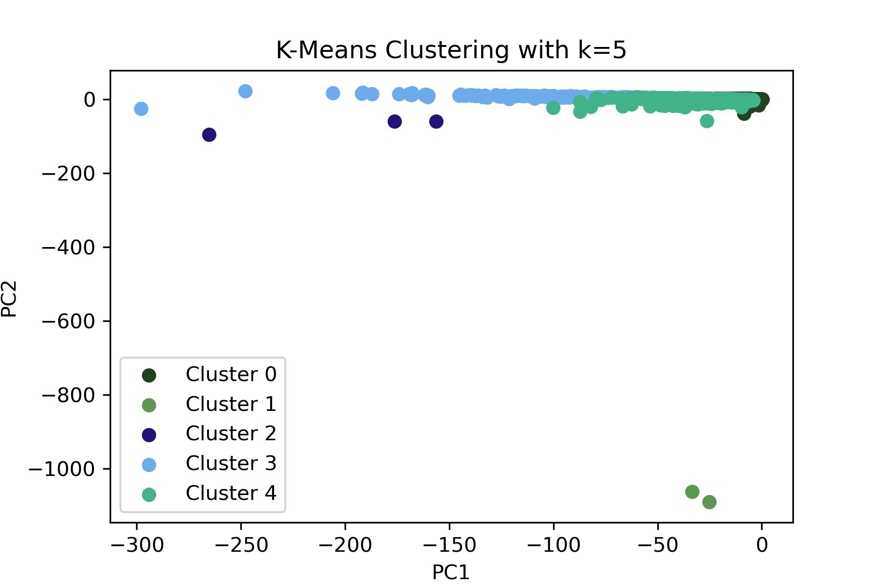 --><imgsrc="images/kmeans_k_5.jpeg"style="width: 70%; height: auto;"/>In this plot where k=3, there are 3 clusters. The distribution is similar to above with k=5, but clusters 0, 3, and 4 from the previous analysis have been combined into a single cluster (cluster 2) here. This could suggest that the distinctions between these clusters were not 100% accurate, and they might represent small differences of a similar topic. As seen with the sillouette scores, a k=3 could imply that while increasing the number of clusters provides more granularity, it may also introduce some overlap/less clear separation between the clusters so k=3 is most likely a better choice in this case. Futhermore, when comparing to the LDA topic number choices above, a lower number had less overlap in words compared to a higher number supporting the choice of a lower k value.<!-- 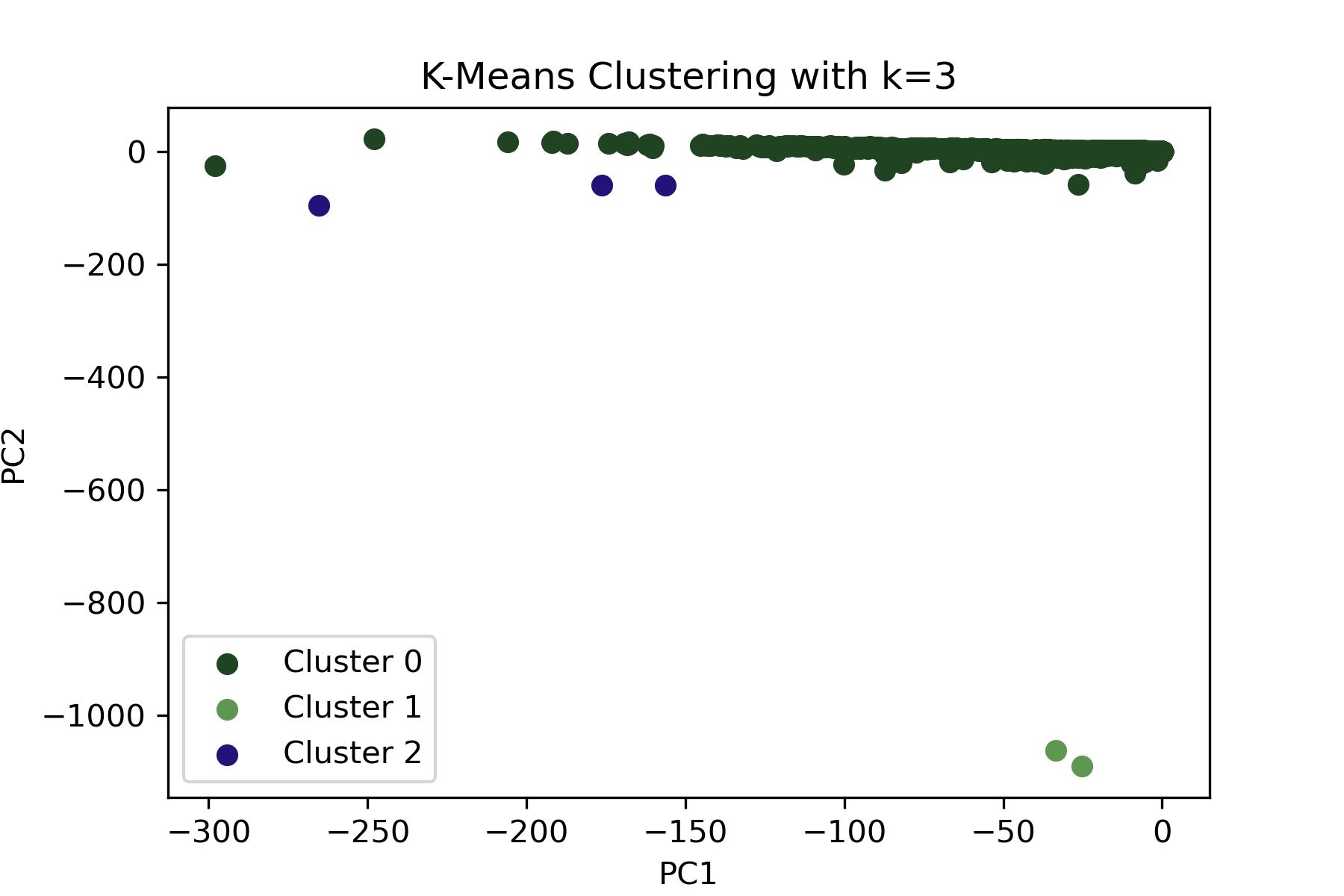 --><imgsrc="images/kmeans_k_3.jpeg"style="width: 70%; height: auto;"/>### Summary and Concluding ThoughtsNaive Bayes, LDA, and K-Means Clustering were performed to answer the project's last three business topics. The text classification showed promise for accurately identifying the usefulness of Reddit posts in the context of job searching and interview help. In labeling the posts, it was surmised that the highest representation in the data consists of posts with low usefulness, followed by roughly equal representation between high and medium levels of usefulness. This is because many of the posts might not bring new relevant information but instead can be something along the lines of 'good post', or 'makes sense'. While these would likely be comments, they are still part of the analysis. The model can predict posts with either high usefulness or low usefulness relatively well, but struggles to predict posts with medium usefulness. This is likely due to the somewhat arbitrary nature of the system used to label the posts. Given a more robust system for labeling the usefulness of the Reddit posts, this model could realistically help job-seekers to find Reddit users' most useful firsthand accounts of interview experiences and advice in realtime. In terms of the meaning of the three significant LDA topics, there is a clear distinction between what each of them contains. The first topic includes keywords such as interview, job, company, and others. Therefore, posts associated with this topic will simply provide non-technical information about the companies and other related topics. The second topic encompasses subjects such as array, gt, code, int, and others; this is the more technical topic, so it is expected to yield specific technical advice or questions. Lastly, the third topic is a more generalized version of the second, with keywords such as problems, leetcode, questions, solve, problem, and others. This is expected to pertain to specific questions that are asked in a technical interview and the solutions desired. Being able to divide the posts into these 3 topics and classify novel posts with a predicted level of usefulness provides significant information, producing a narrative encompassing the essence of the Reddit posts. Such analysis is extremely useful not only to job seekers but also to the HR teams of different companies to help determine what needs to be improved in their hiring process.From the figures above, visible clusters have been dectected. In this case, it is hard to say what these clusters represent with confidence, because the algorithm created the groups based on the text input. Nevertheless, more distinct clusters can be seen when k=3, which potentially means looking at 3 different features of the dataset. Similar results arose with the LDA analysis: when the number of topics being analyzed was 3, better results were produced. Therefore, it can be assumed that the clusters in this case represent number of categories, and the optimal number of cluster is 3.</div>[^1]: Source: [Medium](https://medium.com/@connectwithghosh/topic-modelling-with-latent-dirichlet-allocation-lda-in-pyspark-2cb3ebd5678e).
Machine Learning
The goal of this part of the project is to improve the content relevance and user engagement with posts related to technical interviews on Reddit. By leveraging machine learning models such as Latent Dirichlet Allocation (LDA), which assigns a topic to each post, and K-Means clustering, showing us the different possible groupings based on a selected number of features chosen to group by, a clear analysis of the distribution of posts can be achieved. By utilizing the machine learning technical topics described on the home page, the topics associated with the different Reddit posts were found and able to be divided into 3 different categories, seemingly the most efficient number of categories given the data. A machine learning model was built to classify the usefulness of Reddit posts into groups of low, medium, or high usefulness based on upvote score, comment count, and text length.
Topic 8: Text Classification
Goal: Label posts as useful, semi-useful, or not useful through the use of text classification to provide job seekers guidance as to which characteristics contribute to a post’s engagement and, therefore, which discussions are most valuable for their study and preparation, allowing for focus on high-value content or shifting their focus elsewhere accordingly.
1) Determine Labels for Text Classification
As mentioned previously, the goal is to build a model that will identify novel Reddit posts and comments as useful, semi-useful, or not useful. In order to accomplish this, labels need to be assigned to the preexisting data. A usefulness label will be assigned to a comment or submission based on the following criteria:
Upvote/downvote score
This is possibly the best metric for measuring post usefulness. However, the meaning of an upvote on Reddit is oftentimes unclear. Upvotes are sometimes given to thank useful comments/submissions, but other times they’re given as kudos to funny or clever comments/submissions. Therefore, by themselves they are not an ideal measure of usefulness.
Number of comments
In the case of submissions, this metric signifies the number of comments addressing the submission. For for comments themselves, this metric signifies the number of other comments addressing the same submission. This serves as a proxy for the importance of the overall discussion.
Length of text
As mentioned previously, upvotes are sometimes given as appreciation for witty or ironic comments that are not useful by the team’s standards. These types of comments are often very short, so incorporating the length of the text into the label assignments will sift out comments that aren’t useful and help ameliorate that problem.
The first part in assigning the labels is to rescale each of these three variables from 0 to 1 using the following code:
Code
# Scale score, comment_count, and text_length to 0 to 1# Code referenced from https://stackoverflow.com/a/56953290/17331025from pyspark.ml.feature import MinMaxScalerfrom pyspark.ml.feature import VectorAssemblerfrom pyspark.ml import Pipelinefrom pyspark.sql.types import DoubleTypedf_scaled = df.alias('df_scaled')# UDF for converting column type from vector to double typeunlist = f.udf(lambda x: round(float(list(x)[0]),3), DoubleType())# Iterating over columns to be scaledfor i in ["score","comment_count", "text_length"]:# VectorAssembler Transformation - Converting column to vector type assembler = VectorAssembler(inputCols=[i],outputCol=i+"_vect")# MinMaxScaler Transformation scaler = MinMaxScaler(inputCol=i+"_vect", outputCol=i+"_scaled")# Pipeline of VectorAssembler and MinMaxScaler pipeline = Pipeline(stages=[assembler, scaler])# Fitting pipeline on dataframe df_scaled = pipeline.fit(df_scaled).transform(df_scaled).withColumn(i+"_scaled", unlist(i+"_scaled")).drop(i+"_vect")
Now, arbitrary weights are defined to assign to each of the three rescaled variables based on the subjective perception of the extent to which each one contributes to the overall usefulness of a submission or comment. The weights are designed as follows:
1.0 for score since it is considered to be the most important
0.8 for comment count it is considered to be somewhat important
0.5 for text length since is it considered to be the least important
Thus, a “label metric” is defined with the following formula:
# Define arbitrary weights for each of the three variables:lab_weights = [1, .8, .5] df_lab = df_scaled.withColumn('lab_metric', f.lit(lab_weights[0]) * f.col('score_scaled') + f.lit(lab_weights[1]) * f.col('comment_count_scaled') + f.lit(lab_weights[2]) * f.col('text_length_scaled'),)df_lab.select('lab_metric').summary().show()
summary
lab metric
Count
128345
Mean
0.3089
Standard Deviation
0.1178
Minimum
0.2092
25%
0.2376
50%
0.2662
75%
0.3324
Maximum
1.7658
Based on the summary statistics of this label metric, the labels will be assigned according to these thresholds:
Label
Metric
2 - High usefulness/popularity
Greater than 0.3324
1 - Medium usefulness/popularity
Between 0.2662 and 0.3324
0 - Low usefulness/popularity
Less than 0.2662
These thresholds roughly correspond to the 50th and 75th percentiles of the label metric. The rationale behind this decision is that Reddit is generally filled with many low-effort submissions and comments. The conservative assumptions are that about 50% of all submissions and comments will have low usefulness, 25% will have high usefulness, and the other 25% percent will be somewhere in the middle. The label metric calculated above is being used to assign these labels accordingly.
The majority of the text cleaning was performed during the NLP phase, so at this point the only cleaning needed is to separate the text by whitespace and remove stopwords. In the code below, the pipeline is defined, a train-test split is performed, the model is trained, and six different values (0.0, 0.2, 0.4, 0.6, 0.8, 1.0) for the Naive Bayes smoothing hyperparameter \(\alpha\) are tested.
Code
# This code was composed with the help of ChatGPT (primarily for identifying proper syntax)# Import librariesfrom pyspark.ml import Pipelinefrom pyspark.ml.feature import RegexTokenizer, StopWordsRemover, CountVectorizer, IDFfrom pyspark.ml.classification import NaiveBayesfrom pyspark.ml.evaluation import MulticlassClassificationEvaluatorfrom pyspark.ml.tuning import ParamGridBuilder, CrossValidator# Tokenizetokenizer = RegexTokenizer(inputCol="clean_body", outputCol="words", pattern="\\W")# Remove stopwordsstop_words_remover = StopWordsRemover(inputCol="words", outputCol="filtered_words")# TF-IDF vectorizationcv = CountVectorizer(inputCol="filtered_words", outputCol="raw_features")idf = IDF(inputCol="raw_features", outputCol="features")# Naive Bayes modelnb = NaiveBayes()# Pipelinepipeline = Pipeline(stages=[tokenizer, stop_words_remover, cv, idf, nb])# Train-test splittrain_data, test_data = df_model.randomSplit([0.8, 0.2], seed=123)# Hyperparameter tuning - test different alphas (smoothing parameter)paramGrid = (ParamGridBuilder() .addGrid(nb.smoothing, [0.0, 0.2, 0.4, 0.6, 0.8, 1.0]) .build())evaluator = MulticlassClassificationEvaluator(labelCol="label", predictionCol="prediction", metricName="accuracy")crossval = CrossValidator(estimator=pipeline, estimatorParamMaps=paramGrid, evaluator=evaluator, numFolds=5)# Fit modelcv_model = crossval.fit(train_data)# Make predictionspredictions = cv_model.transform(test_data)# Get accuracy and f1 scoreaccuracy = evaluator.evaluate(predictions)f1_score = MulticlassClassificationEvaluator(labelCol="label", predictionCol="prediction", metricName="f1").evaluate(predictions)print(f"Accuracy: {accuracy}")print(f"F1 Score: {f1_score}")
3) Evaluate model
The final performance of the model yields a validation accuracy of 0.5011 and F1 score of 0.4948. While these metrics indicate better performance than random guessing (which would, for example, theoretically produce an accuracy of 0.33), it is important to bear in mind that the system used for assigning labels is not perfect. The importance labels to the comments and submissions were assigned based on the team’s own understanding of how Reddit works and what useful posts typically look like. This was a necessary approach given the scale of data, but if there was more time and resources, labels would most likely be manually assigned in order to ensure optimal performance in identifying useful posts. If this model were to be used in a practical application (for instance, to search Reddit for new posts that may be useful to job candidates), then the alternative approach of manually labeling each post in the training set would be preferred.
The confusion matrix above further supports the need for a more robust system of labeling comments and submissions. The model predicts low-importance posts and high-importance posts relatively well, but clearly struggles at predicting semi-important posts. This is likely because the labeling system used left the semi-important label somewhat ambiguous. Where the low-importance and high-importance labels likely had their own distinct tokens to distinguish those labels, the posts labeled as semi-important likely had a mix of the two.
Topic 9: Topic Modeling
Goal: Enhance the understanding of content themes in technical interview subreddits by applying Latent Dirichlet Allocation (LDA). This goal focuses on extracting concise and meaningful topics from the large amounts of text data from reddit, revealing trends in online discussions surrounding technical interviews.
To find the clusters of the reddit post text data, an unsupervised learning technique may be used. LDA (Latent Dirichlet Allocation) is a popular unsupervised topic modeling method. With LDA, each “document”, a post in this case, is assigned a “topic”. Topics are comprised of several words that have associated weights. The weights are how likely the words belong to the gieven topic. Words with higher weights are the more “dominant” keywords for the given topic.
As seen in the EDA section of this website, the reddit data was filtered on 7 “subreddits”, essentially topics themselves. Can unsupervised machine learning produce similar topics, or do new topics arise? First, an LDA model with 7 topics will be trained to see how the topics compare to the subreddit topics and if any other noteable relationships arise. After this, LDA models with different amounts of topics will be trained to see if better results could be obtained.
Topic 7: solution, removed, question, problem, time, test, design, cases, dp, system
It is clearly difficult to distinguish the topics as many contain the same and/or similar topic terms. The LDA was able to group the text into more general interview topics and more technical topics. For example, topics 2, 3 and 5 are the most technical topics out of the 7 with keywords like “leetcode” (one of the subreddits), “solution”, “problem”, “array”, “function”, etc. Topic 3 appears more general than topics 2 and 5. Topic 5 has a higher chance of having more detailed key words such as “algorithms” and “programming” while topic 2 contains keywords like “int”, “array”, “function”, “list”, “node”, etc. Clearly, topic 2 would contain posts that are about specific coding problems that work with these data structures. Topic 1 contains the keywords “job”, “offer”, “company”, “position”, and “salary”. Posts in this topic appear to be more about the logistics of interviewing - possibly questions about companies and the salaries of various positions, navigating accepting/declining a job offer, etc. Topics 4 and 6 appear to contain posts that are more about general interviewing, which is not surprising as a general “interviews” subreddit was used to filter the raw dataset. It is more difficult to differentiate between these two topics however. Topic 7 is similar to topics 4 and 6 but contains keywords “test”, “design”, and “cases”, so this topic may contain posts that are more related to case interviews, test questions for interviews, etc. The plot below shows the top 10 keywords in each of the 7 topics. The bars represent each term’s weight and are sorted from greatest to least.
From the discussion above, it is clear that topic modelling with LDA can be challenging, especially with multiple topics that appear very similar. This unsupervised learning is an effective way to get more insight into the dataset, however, especially a dataset that may not be labelled in any way beforehand.
Code
# Import packagesimport timeimport sagemakerimport numpy as npimport pandas as pdimport pyarrow as paimport pyarrow.dataset as dsimport matplotlib.pyplot as pltimport pyLDAvis.gensim_models as gensimvisfrom gensim import corpora, modelsfrom s3fs import S3FileSystemfrom pyspark.sql import SparkSessionfrom pyspark.sql.functions import udffrom pyspark.sql.types import ArrayType, StringType, IntegerTypefrom sagemaker.spark.processing import PySparkProcessorfrom pyspark.ml.feature import Tokenizer, CountVectorizer, IDF, PCA, StopWordsRemoverfrom pyspark.ml.clustering import KMeans, LDAfrom pyspark.ml import Pipeline# Build Spark sessionspark = ( SparkSession.builder.appName("PySparkApp") .config("spark.jars.packages", "org.apache.hadoop:hadoop-aws:3.2.2") .config("fs.s3a.aws.credentials.provider","com.amazonaws.auth.ContainerCredentialsProvider", ) .getOrCreate())%%timesession = sagemaker.Session()#s3://sagemaker-us-east-1-131536150362/project/data_reformat_clean_nlp.parquet/bucket ="tm1450-project"output_prefix_data_submissions ="data_reformat_clean.parquet/"s3_path =f"s3a://{bucket}/{output_prefix_data_submissions}"print(f"reading data from {s3_path}")df = spark.read.parquet(s3_path, header=True)print(f"shape of the dataframe is {df.count():,}x{len(df.columns)}")## PREPARE THE DATA# Tokenize the texttokenizer = Tokenizer(inputCol ="clean_body", outputCol ="clean_body_tokenized")tokenized_df = tokenizer.transform(df)# Load english stopwordsstop_words = StopWordsRemover.loadDefaultStopWords("english")extra_stopwords = ["dont", "im", "a", "b", "c", "d", "e", "f", "g", "h", "i", "j", "k", "l", "m", "n", "o", "q", "r", "s", "t", "u", "v", "w", "x", "y", "z", "0", "1", "2", "3", "4", "5", "6", "7", "8", "9"]# Remove stop words from tokenized columnstop_remover = StopWordsRemover(inputCol ="clean_body_tokenized", outputCol ="clean_body_no_stop", stopWords = stop_words+extra_stopwords)tokenized_df_no_stop = stop_remover.transform(tokenized_df)# Vectorize the columncount_vectorizer = CountVectorizer(inputCol ="clean_body_no_stop", outputCol ="cv_features", vocabSize =5000, minDF =10.0)cv_model = count_vectorizer.fit(tokenized_df_no_stop)vocabulary = cv_model.vocabulary # Store the vocabularycv_df = cv_model.transform(tokenized_df_no_stop)# TF-IDFidf = IDF(inputCol ="cv_features", outputCol ="features")idf_model = idf.fit(cv_df)final_df = idf_model.transform(cv_df) ## FIT LDA MODEL AND GET THE TOPICSnum_topics =7# Define model with num_topics and fitlda = LDA(k = num_topics, maxIter =100)lda_model7 = lda.fit(final_df.select("features"))lda_df7 = lda_model7.transform(final_df)# View resultstopics7 = lda_model7.describeTopics(maxTermsPerTopic =10)topics7.show(truncate =True)# Get the keywords for each of the topicskeywords_by_topic7 = topics7.rdd.map(lambda row: row["termIndices"]).map(lambda indices: [vocabulary[idx] for idx in indices]).collect()# Get the term weights for each topicterm_weights_by_topic7 = topics7.select("termWeights").rdd.flatMap(lambda x: x).collect()# Print out the keywords by topicfor i, words inenumerate(keywords_by_topic7):print(f"Topic {i+1}: {', '.join(words)}") # Plotting keywords for each topicplt.figure()for i inrange(num_topics): plt.subplot(((num_topics +4-1)//4), 4, i +1) plt.barh(range(len(keywords_by_topic7[i])), term_weights_by_topic7[i], color ="#251279", alpha =1) plt.yticks(range(len(keywords_by_topic7[i])), keywords_by_topic7[i]) plt.title(f"Topic {i+1}") plt.xlabel("Keyword") plt.gca().invert_yaxis()plt.tight_layout()# Save figureplt.savefig('../../website-source/images/lda_plot_7_topics.png', dpi =300)plt.show()
LDA with 3 Topics
Now, the LDA will be trained with fewer topics to see if it becomes easier to differentiate between the topics.
With only 3 topics, it is clearly easier to distinguish between topics. The set of likely keywords in topic 1 show that posts classified into this topic are most likely about general interview questions, interview advice, discussion about companies in the industry, and more. Topic 2 on the other hand contains more technical keywords such as “int”, “array”, “solution”, and “code.” This topic probably contains posts about specific coding interview/assessment questions. Topic 3 is also technical, but more general than topic 2, containing likely keywords such as “leetcode” (one of the subreddits), “questions”, “solve”, “algorithms”, “learn.” Posts under this topic are probably also asking about coding interviews, what questions may come up, the best ways to prepare and “learn”, etc. Leetcode is a popular website to practice for coding interviews, so this makes sense.
Code
num_topics =3# Define model with num_topics and fitlda = LDA(k = num_topics, maxIter =100)lda_model3 = lda.fit(final_df.select("features"))lda_df3 = lda_model3.transform(final_df)# View resultstopics3 = lda_model3.describeTopics(maxTermsPerTopic =10)topics3.show(truncate =True)# Get the keywords for each of the topicskeywords_by_topic3 = topics3.rdd.map(lambda row: row["termIndices"]).map(lambda indices: [vocabulary[idx] for idx in indices]).collect()# Get the term weights for each topicterm_weights_by_topic3 = topics3.select("termWeights").rdd.flatMap(lambda x: x).collect()# Print out the keywords by topicfor i, words inenumerate(keywords_by_topic3):print(f"Topic {i+1}: {', '.join(words)}") # Plotting keywords for each topicplt.figure()for i inrange(num_topics): plt.subplot(((num_topics +4-1)//4), 4, i +1) plt.barh(range(len(keywords_by_topic3[i])), term_weights_by_topic3[i], color ="#251279", alpha =1) plt.yticks(range(len(keywords_by_topic3[i])), keywords_by_topic3[i]) plt.title(f"Topic {i+1}") plt.xlabel("Keyword") plt.gca().invert_yaxis()plt.tight_layout()# Save figureplt.savefig('../../website-source/images/lda_plot_3_topics.png', dpi =300)plt.show()
Ultimately, LDA is a fantastic way to initially organize a dataset into different topics. In this case, LDA was performed to see if the learned topics were similar to the subreddits used to initially filter the dataset. Additionally, there was a desire to test if any new topics arise.
The topics do seem to align with the subreddits: more general subreddits such as “interview” and “InterviewTips” and more technical/specific subreddits such as “leetcode” and “codinginterview.” Similar categorizations were seen in the learned topics from LDA. As the subreddits used to filter the data were already very specific to interviews, in particular technical and coding interviews, no new topics appeared to arise through LDA.
Topic 10: Post Clustering
Goal: Discover underlying themes in subreddit discussions by applying K-means clustering. This method aims to segment posts and comments into distinct clusters based on the content of the text. This presents an opportunity to offer a new perspective on strong topics and conversation patterns within the technical interview reddit community.
The code below performs text data processing and K-means clustering analysis using Apache Spark in a SageMaker environment. The data read in from s3 undergoes pre-processing, where the ‘clean_body’ reddit text column is tokenized using the Tokenizer module, creating a new column with tokenized text. Subsequently, a CountVectorizer is applied to transform these tokens into a vector of term frequencies (TF), followed by the application of the IDF (Inverse Document Frequency) module, converting the TF vectors into TF-IDF features. These features serve as inputs for the K-means clustering model. K-means is performed for different numbers of clusters, and the resulting clusters are visualized in 2 dimensions using PCA. A function was built to encapsulate all of the prior steps and ends with visualizing the results as you can see below.
The table below presents the silhouette scores for K-means clustering with two different numbers of clusters: 3 and 5. The silhouette score measures how similar an object is to its own cluster compared to other clusters, with a score range from -1 to 1. The clustering with 3 clusters (k=3) achieved a very high silhouette score of approximately 99%. This indicates that the clusters are well-separated. On the other hand, increasing the number of clusters to 5 (k=5) resulted in a lower score of about 90%. Although this is still high, it indicates less distinct clustering compared to the 3-cluster scenario.
k
Silhouette Score
3.0
0.998
5.0
0.902
In the plot below, there are 5 distinct clusters. This may indicate that the reddit dataset has a variety of topics or types of posts that can be separated into 5 groups. However, clusters 2, 3, and 4 seem to be very close to one another, potentially indicating that while the model has assigned them different cluster labels, their distinctions might not be significant and there could be overlap. Cluster 1 is small and separate from the other clusters, which could suggest a niche topic. The largest clusters are 2 and 3 and are spread across a wide range of values for PC1 but a narrow range in terms of PC12. This may suggest a large number of posts share a common theme but vary slightly in that theme.
In this plot where k=3, there are 3 clusters. The distribution is similar to above with k=5, but clusters 0, 3, and 4 from the previous analysis have been combined into a single cluster (cluster 2) here. This could suggest that the distinctions between these clusters were not 100% accurate, and they might represent small differences of a similar topic. As seen with the sillouette scores, a k=3 could imply that while increasing the number of clusters provides more granularity, it may also introduce some overlap/less clear separation between the clusters so k=3 is most likely a better choice in this case. Futhermore, when comparing to the LDA topic number choices above, a lower number had less overlap in words compared to a higher number supporting the choice of a lower k value.
Summary and Concluding Thoughts
Naive Bayes, LDA, and K-Means Clustering were performed to answer the project’s last three business topics. The text classification showed promise for accurately identifying the usefulness of Reddit posts in the context of job searching and interview help. In labeling the posts, it was surmised that the highest representation in the data consists of posts with low usefulness, followed by roughly equal representation between high and medium levels of usefulness. This is because many of the posts might not bring new relevant information but instead can be something along the lines of ‘good post’, or ‘makes sense’. While these would likely be comments, they are still part of the analysis. The model can predict posts with either high usefulness or low usefulness relatively well, but struggles to predict posts with medium usefulness. This is likely due to the somewhat arbitrary nature of the system used to label the posts. Given a more robust system for labeling the usefulness of the Reddit posts, this model could realistically help job-seekers to find Reddit users’ most useful firsthand accounts of interview experiences and advice in realtime.
In terms of the meaning of the three significant LDA topics, there is a clear distinction between what each of them contains. The first topic includes keywords such as interview, job, company, and others. Therefore, posts associated with this topic will simply provide non-technical information about the companies and other related topics. The second topic encompasses subjects such as array, gt, code, int, and others; this is the more technical topic, so it is expected to yield specific technical advice or questions. Lastly, the third topic is a more generalized version of the second, with keywords such as problems, leetcode, questions, solve, problem, and others. This is expected to pertain to specific questions that are asked in a technical interview and the solutions desired. Being able to divide the posts into these 3 topics and classify novel posts with a predicted level of usefulness provides significant information, producing a narrative encompassing the essence of the Reddit posts. Such analysis is extremely useful not only to job seekers but also to the HR teams of different companies to help determine what needs to be improved in their hiring process.
From the figures above, visible clusters have been dectected. In this case, it is hard to say what these clusters represent with confidence, because the algorithm created the groups based on the text input. Nevertheless, more distinct clusters can be seen when k=3, which potentially means looking at 3 different features of the dataset. Similar results arose with the LDA analysis: when the number of topics being analyzed was 3, better results were produced. Therefore, it can be assumed that the clusters in this case represent number of categories, and the optimal number of cluster is 3.


